Data Driven Science & Engineering - Machine Learning, Dynamical Systems, and Control

Part of the Embedded.fm Bookclub
Book Link

Chapter 1 Dimensionality Reduction and Transforms

The SVD provides a stable matrix decomposition that is guaranteed to exist and can me used for many purposes
The SVD can be used to obtain "low-rank" approximations to matrices and perform pseudo inverses of non-square matrices to find a solution to a system of equations $A x = b$
The SVD can also be used as the underlying algo of principal component analysis which allows high-dimensional data to be composed into statistically descriptive factors

The SVD generalizes the concept of the Fast Fourier Transform. While the FFT works in idealized settings, the SVD is a more generic data-driven technique. The SVD may be thought of as providing a basis that is tailored to specific data, as opposed to the FFT which provides a generic basis

In many domains, systems generate data that is a natural fit for large matrices or arrays. EG: a time series of data from an experiment could be arranged into a matrix with each column containing all of the measurements from time $T$ . If the data at each instant is multi-dimensional, such as in 3d weather simulations, it's possible to flatten this data into a high-dimensional column vector forming the columns of a large matrix.

The Data generated by these systems are low rank which means there are jus a few dominant patterns that explain high-dimensional data. The SVD is an efficient method of extracting these patterns

Overview

The SVD Provides a systematic way to determine a low-dimensional approximation to high-dimensional data in terms of dominant patterns.
The SVD is GUARANTEED to exist for any matrix

The SVD an help compute a pseudo-inverse of a non-square matrix which can give us solutions to under or overdetermined matrix equations
The SVD can also be used to de-noise datasets.
The SVD can also characterize the input and output geometry of a linear map between vector spaces.

SVD Definition

Generally we're interested in analyzing a large data set $X \in C^{n \times m},$

X = [\begin{matrix} | & | & | \\ x_{1} & x_{2} & \dots & x_{m} \\ | & | & | \end{matrix}]

The columns $x_{k} \in C^{n}$ may be measurements from simulations or experiments.
The index $k$ is a label indicating the $k^{t h}$ distinct set of measurements. In this book, $X$ will be time-series data and $x_{k} = x (k Δ t)$
In many cases, the state dimension is large (ie millions or billions of DOF). The columns can be thought of as "snapshots" and $m$ is the number of snapshots in $X$ . For many systems $n ≫ m$ which gives us a "tall-skinny" matrix as opposed to a "short-fat" matrix where $n ≪ m$ .

The SVD is a unique matrix decomp that exists for every complex valued matrix $X \in C^{n \times m},$

X = U Σ V *

$U \in C^{n \times m}$ and $V \in C^{n \times m}$ are unitary matrices and $Σ \in R^{n \times m}$ is a matrix with real, non-negative entries on the diagonal and zeros off the diagonal. Here $*$ denotes the complex conjugate

The condition that $U$ and $V$ are unitary is used often

When $n \geq m$ the matrix $Σ$ has AT MOST $m$ non-zero elements on the diagonal and may be written as $Σ = [\begin{matrix} \hat{Σ} \\ 0 \end{matrix}] .$ This means we can exactly represent $X$ using the economy SVD

X = U Σ V^{*} = [\begin{matrix} \hat{U} & {\hat{U}}^{⊥} \end{matrix}] [\begin{matrix} \hat{Σ} \\ 0 \end{matrix}] V^{*} = \hat{U} \hat{Σ} V^{*} .

The columns of ${\hat{U}}^{⊥}$ span a vector space that is complementary and orthogonal to $\hat{U}$ . The columns of $U$ are the left singular vectors of $X$ and the columns of $V$ are right singular vectors.
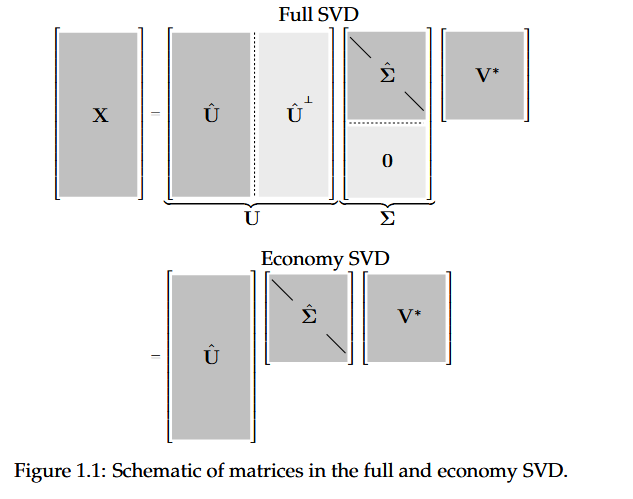
Diagonal elements of $\hat{X} \in C^{n \times m},$ are called singular values and are ordered large to small. Rank $X$ is equal to the quantity of non-zero singular values

Computing the SVD

import numpy as np
X=  np.random.rand(5,3)  #Create a random data matrix
U,S,V = np.linalg.svd(X,full_matrices=True) #Full SVD
Uhat, Shat,Vhat = np.linalg.svd(X, full_matrices=False) #Economy SVD

1.2 Matrix Approximation

Glossary

Term	Definition
SVD	Singular Value Decomposition
PCA	Principal Component Analysis